
library(isoformic)

extdata <- fs::path_package("isoformic", "extdata")
annot_dir <- prepare_isoformic_annotation(download_reference(version = "33", file_type = "gff"))
iso <- IsoformicExperiment(
  experiment_name = "preeclampsia_placenta",
  annot_path = annot_dir,
  assays = list(abundance = read_parquet(fs::path(extdata, "pe_abundance.parquet"))),
  col_data = read_parquet(fs::path(extdata, "pe_col_data.parquet"))
)
de_tx(iso) <- read_parquet(fs::path(extdata, "pe_det.parquet"))
de_gene(iso) <- read_parquet(fs::path(extdata, "pe_deg.parquet"))Three plots show a gene and its isoforms from three angles: the fold-change of each isoform next to that of the gene, the expression of each isoform across conditions and the exon-intron structure of each isoform along the genome. All of them are ggplot2 objects and take an IsoformicExperiment (or the equivalent table, see working with plain tables).
They start from the object built in the introduction:
Log2 fold-change plot
plot_log2fc() compares the fold-change of a gene with that of each of its transcripts, coloured by transcript type and faded when not significant. Several genes give one panel each.
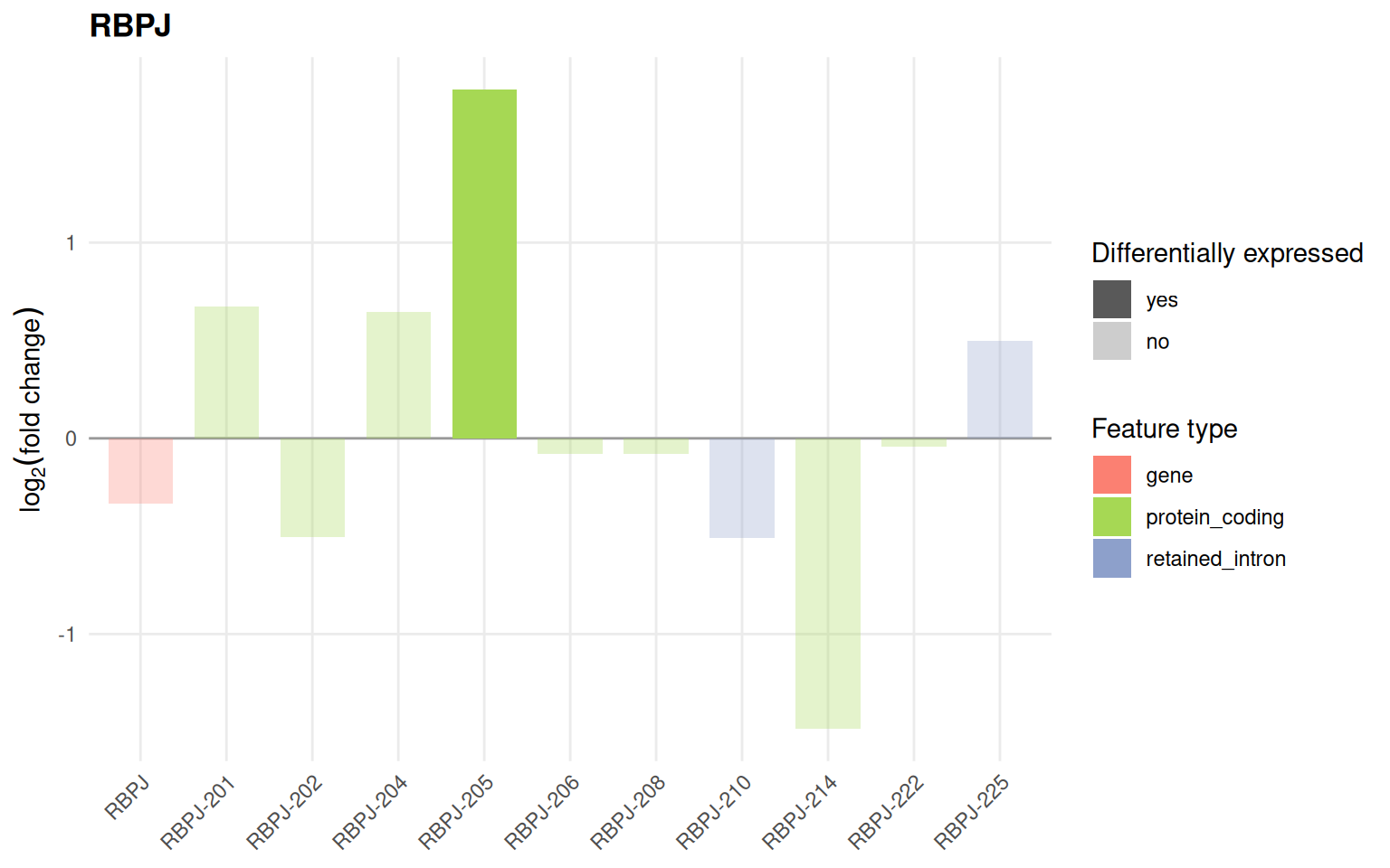
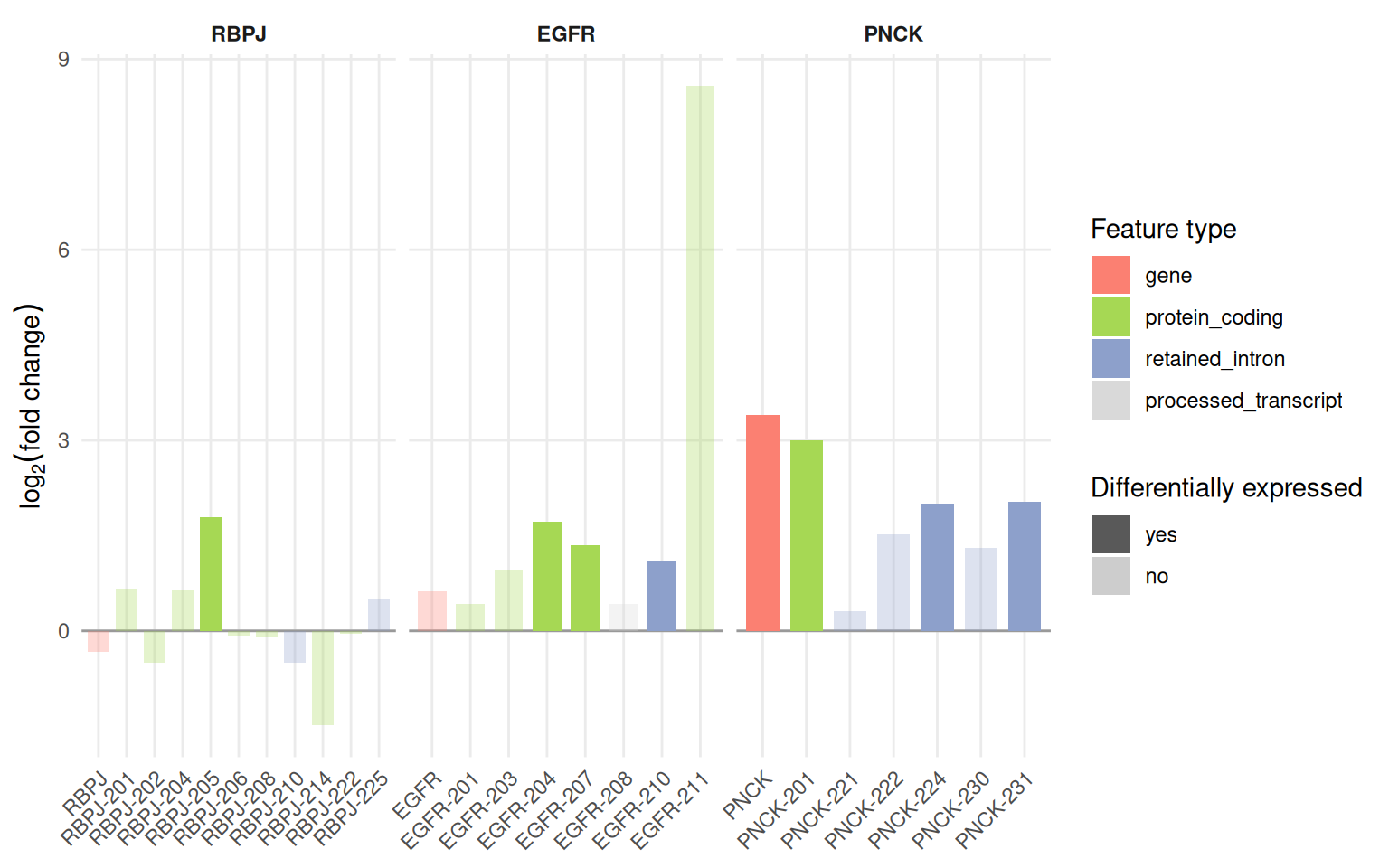
The colours come from tx_type_palette() and can be replaced through the tx_type_palette property of the object; productivity_palette() colours the productivity classes the same way.
tx_type_palette()
#>                               gene                     protein_coding
#>                          "#fb8072"                          "#a6d854"
#>                    retained_intron     protein_coding_CDS_not_defined
#>                          "#8da0cb"                          "#fc8d62"
#>            nonsense_mediated_decay                             lncRNA
#>                          "#66c2a5"                          "#e78ac3"
#>               processed_pseudogene transcribed_unprocessed_pseudogene
#>                          "#ffd92f"                          "#e5c494"
#>             unprocessed_pseudogene                     non_stop_decay
#>                          "#d9d9d9"                          "#d9d9d9"
#>     transcribed_unitary_pseudogene                         pseudogene
#>                          "#d9d9d9"                          "#ffffb3"
#>                 unitary_pseudogene               processed_transcript
#>                          "#d9d9d9"                          "#d9d9d9"
#>                            unknown                              novel
#>                          "#bdbdbd"                          "#8c6bb1"
#>                           misc_RNA                              miRNA
#>                          "#d9d9d9"                          "#d9d9d9"
#>                              snRNA                             snoRNA
#>                          "#d9d9d9"                          "#d9d9d9"
#>                  full-splice_match            incomplete-splice_match
#>                          "#a6d854"                          "#66c2a5"
#>                   novel_in_catalog               novel_not_in_catalog
#>                          "#fdb462"                          "#bc80bd"
#>                              genic                          antisense
#>                          "#d9d9d9"                          "#80b1d3"
#>                             fusion                         intergenic
#>                          "#fccde5"                          "#d9d9d9"
#>                       genic_intron                        coding_mRNA
#>                          "#d9d9d9"                          "#a6d854"
#>                  lncRNA_intergenic                   lncRNA_antisense
#>                          "#e78ac3"                          "#8da0cb"
#>                   lncRNA_divergent              lncRNA_sense_intronic
#>                          "#fc8d62"                          "#66c2a5"
#>                  sense_overlap_RNA                        short_ncRNA
#>                          "#ffd92f"                          "#e5c494"
#>                   uncertain_coding
#>                          "#b3b3b3"
Expression profile plot
plot_tx_expr() shows the mean expression of a gene and of each of its isoforms in every condition, with standard deviations, so that isoform switches become visible as crossing lines.
plot_tx_expr(iso, gene_name = "RBPJ", group = "condition")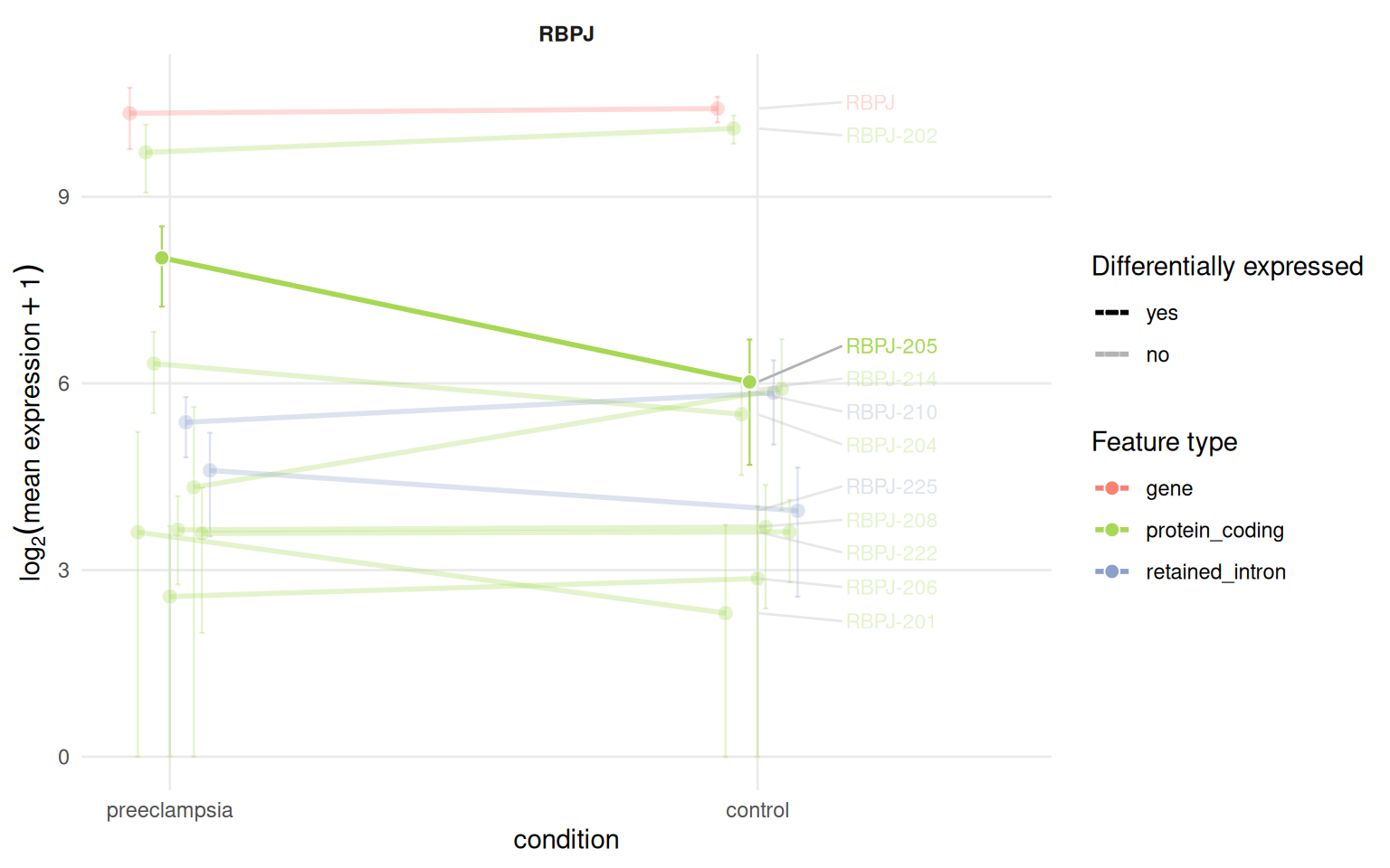
plot_tx_expr(iso, gene_name = c("IL2RA", "EGFR"), group = "condition", ncol = 2)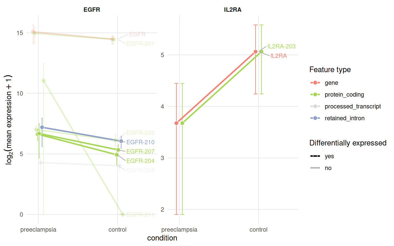
The underlying table is available with profile_data().
head(profile_data(iso, gene_name = "RBPJ", group = "condition"))
#> # A tibble: 6 × 10
#>   feature_id feature_name feature_type gene_id gene_name group mean_expr sd_expr
#>   <chr>      <chr>        <chr>        <chr>   <chr>     <fct>     <dbl>   <dbl>
#> 1 ENSG00000… RBPJ         gene         ENSG00… RBPJ      pree…   1297.    427.
#> 2 ENSG00000… RBPJ         gene         ENSG00… RBPJ      cont…   1367.    195.
#> 3 ENST00000… RBPJ-201     protein_cod… ENSG00… RBPJ      pree…     11.2    25.1
#> 4 ENST00000… RBPJ-201     protein_cod… ENSG00… RBPJ      cont…      3.95    8.30
#> 5 ENST00000… RBPJ-202     protein_cod… ENSG00… RBPJ      pree…    838.    303.
#> 6 ENST00000… RBPJ-202     protein_cod… ENSG00… RBPJ      cont…   1095.    169.
#> # ℹ 2 more variables: n_samples <int>, is_de <chr>
Genomic context plot
plot_genomic_context() draws the exon-intron structure of every annotated isoform of a gene along the genome, coloured by transcript type, labelled with its mean expression and outlined when differentially expressed. Poison exons (see the productivity article) are outlined as well.
plot_genomic_context(iso, gene_name = "FLT1")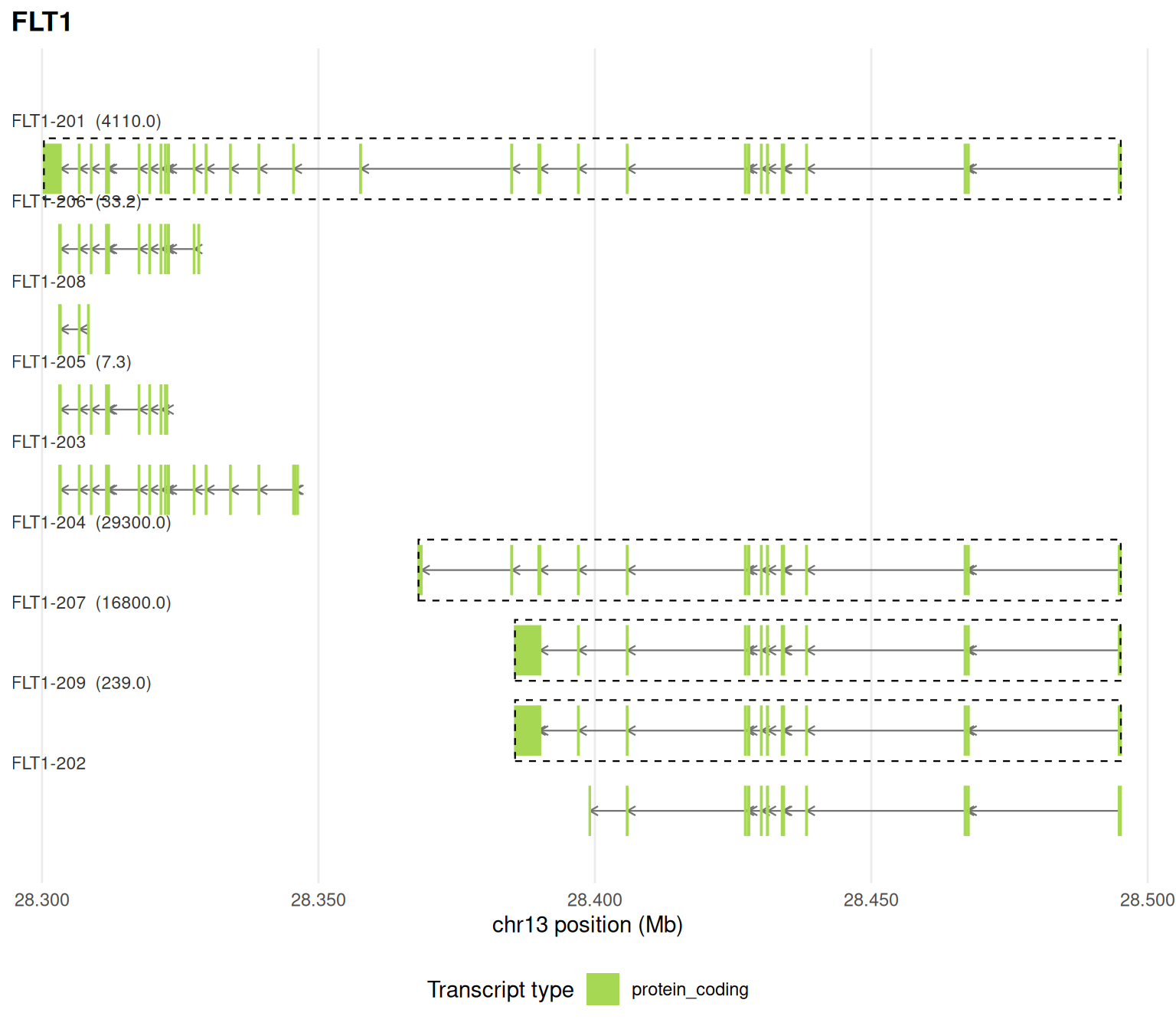
plot_genomic_context(iso, gene_name = "EGFR")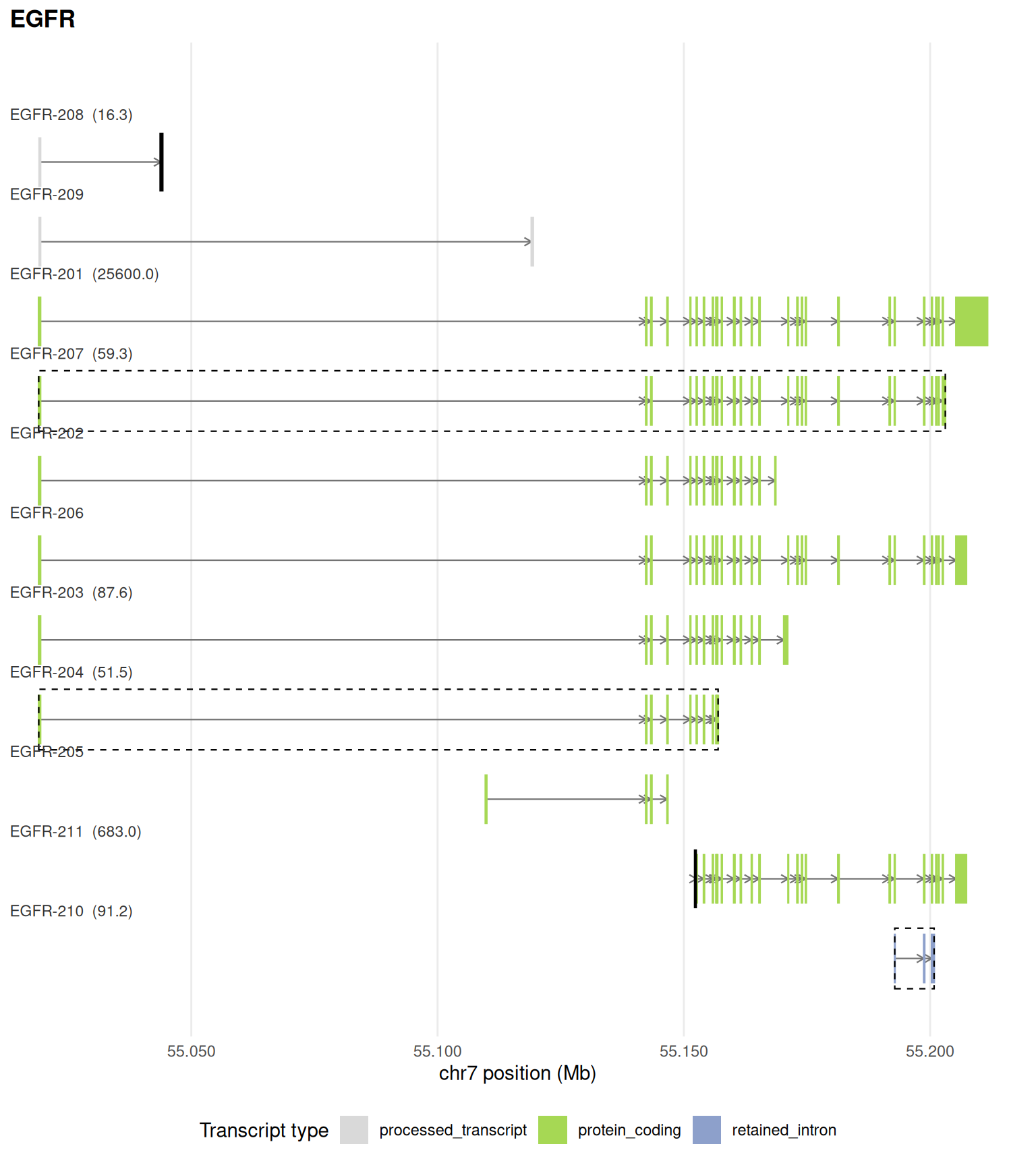
upstream_offset widens the window, for example to show a neighbouring gene:
plot_genomic_context(iso, gene_name = "XIST", upstream_offset = 100000)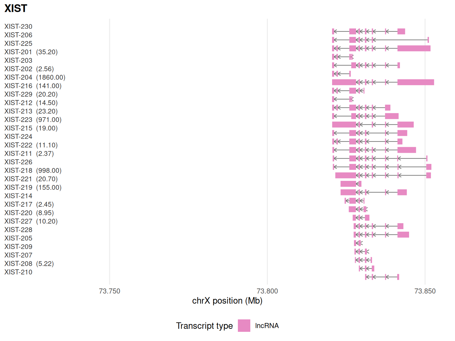
Session information
sessionInfo()
#> R version 4.6.2 (2026-10-29)
#> Platform: x86_64-pc-linux-gnu
#> Running under: Ubuntu 26.04.1 LTS
#>
#> Matrix products: default
#> BLAS:   /usr/lib/x86_64-linux-gnu/openblas-pthread/libblas.so.3
#> LAPACK: /usr/lib/x86_64-linux-gnu/openblas-pthread/libopenblasp-r0.3.32.so;  LAPACK version 3.12.0
#>
#> locale:
#>  [1] LC_CTYPE=C.UTF-8       LC_NUMERIC=C           LC_TIME=C.UTF-8
#>  [4] LC_COLLATE=C.UTF-8     LC_MONETARY=C.UTF-8    LC_MESSAGES=C.UTF-8
#>  [7] LC_PAPER=C.UTF-8       LC_NAME=C              LC_ADDRESS=C
#> [10] LC_TELEPHONE=C         LC_MEASUREMENT=C.UTF-8 LC_IDENTIFICATION=C
#>
#> time zone: UTC
#> tzcode source: system (glibc)
#>
#> attached base packages:
#> [1] stats     graphics  grDevices utils     datasets  methods   base
#>
#> other attached packages:
#> [1] isoformic_0.1.2.9022
#>
#> loaded via a namespace (and not attached):
#>  [1] gtable_0.3.6       jsonlite_2.0.0     dplyr_1.2.1        compiler_4.6.2
#>  [5] tidyselect_1.2.1   Rcpp_1.1.2         scales_1.4.0       yaml_2.3.12
#>  [9] fastmap_1.2.0      ggplot2_4.0.3      R6_2.6.1           labeling_0.4.3
#> [13] generics_0.1.4     curl_8.1.0         knitr_1.52         ggrepel_0.9.8
#> [17] tibble_3.3.1       DBI_1.3.0          pillar_1.11.1      RColorBrewer_1.1-3
#> [21] rlang_1.3.0        utf8_1.2.6         xfun_0.62          fs_2.1.0
#> [25] S7_0.2.2           otel_0.3.0         cli_3.6.6          withr_3.0.3
#> [29] magrittr_2.0.5     digest_0.6.39      grid_4.6.2         lifecycle_1.0.5
#> [33] vctrs_0.7.3        evaluate_1.0.5     glue_1.8.1         farver_2.1.2
#> [37] duckdb_2.0.0       rmarkdown_2.32     tools_4.6.2        pkgconfig_2.0.3
#> [41] htmltools_0.5.9